Ionosphere

The ionospheric solver in GUMICS calculates conductivity, electric potential and currents.

Variables and equations

The ionosphere is modelled in GUMICS as a spherical surface, on which radially integrated current continuity with field-aligned current as source term is imposed:

Here the following variables are used:

Σ is the height-integrated conductivity tensor
Φ is the ionospheric potential
v_n is the neutral wind
j_∥ is the field-aligned current
b⋅r is the cosine of the angle between the magnetic field direction and the radial direction.

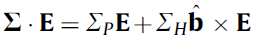
The height-integrated conductivity tensor is defined by its action on any electric field E as

where Σ_P and Σ_H are the Pedersen and Hall conductivity.

Discretisation

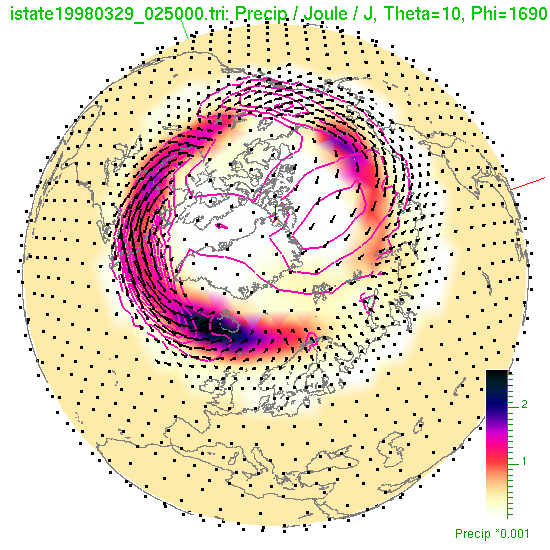
The ionosphere is disctretised with a triangular grid, whose resolution is 360 km in the polar caps and 180 km in the auroral oval. The grid is thus adapted, but the adaptation is not dynamic as in the magnetosphere. The current continuity equation (above) is solved by the conjugate gradient algorithm (Press et al., 1992). As the ionosphere is a spherical surface and is solved in its entirety, it has no boundaries. The only inputs needed by the solver are the solar EUV radiation, the electron precipitation and the field aligned current. The ionosphere is solved every fourth second.

The ionosphere as depicted by the visualisation program ionovis. Colour shows particle precipitation and arrows electric current.

Calculating conductances

The solar EUV contribution to the ionospheric conductances is considered constant in time, but naturally it varies with the solar zenith angle. The empirical formulas by Moen and Brekke (1993) are used. The solar EUV radiation is approximated by the 10.7 cm radio flux (commonly known as F10.7), a widely used proxy solar UV activity, whose standard values is taken to be 100 ⋅ 10⁻²² W/m².

The electron precipitation flux is obtained from the magnetospheric part of the simulation. Its contribution to ionisation is calculated by textbook formulas using collision frequencies from the MSIS model (Hedin 1991). The 3-dimensional conductivity is then height-integrated.

Finally the total conductivity is calculated as the square sum of the electron precipitation and solar UV contributions:

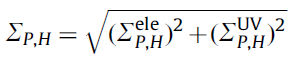
This type of summing is used because the conductivity is proportional to electron density, which in a stationary state is proportional to the square root of the production rate, and it is the production rates that can be summed linearly.

References

Hedin, A.E., 1991. Extension of the MSIS thermospheric model into the middle and lower atmosphere. Journal of Geophysical Research 96, 1159–1172.
Moen, J., Brekke,A., 1993. The solar flux influence on quiet time conductances in the auroral ionosphere. Geophysical Research Letters 20, 971–974.
Press, W.H., Teukolsky, S.A., Vetterling, W.T., Flannery, B.P., 1992. Numerical Recipes in C The art of scientific computing. 2nd ed., Cambridge.